Normalizing Flows, a Simple Example
This post is meant as an exercise in implementing a generative normalizing flows model in a 2D environment. The full notebook can be found on github. It will assume some prior knowledge of Jax/Flax and normalizing flows. You also need to know (or be willing to learn) some fundamental concepts in multi-variable calculus, probabilities, etc. I will cite the resources that I found helpful as needed. Personally, I find it's best to set aside a few days for each topic separately, rather than trying to learn multiple things at once.
To familiarize yourself with Jax/Flax, I would recommend this notebook by University of Amsterdam's Deep learning course (which also has other must read resources included). The Jax documentation is also essential. If you are already familiar with numpy and another deep learning library, learning the basics of Jax should take somewhere between a few hours to a couple of days. To get an understanding of normalizing flows (without reading a 50+ page paper) you can take a look at one or more of the following links:
Lilian Weng's blog: Good rundown of the theory and many of the common functions.
Eric Jang's blog: Theory and a tensor-flow (🤮) implementation. I found the code hard to follow since a lot of magic happens in tensor-flow. Eric has since made a pure Jax tutorial as well, which I highly recommend once you're comfortable with the theory (and if you don't want to bother with flax/optax).
UVADLC notebook: Helpful, but much of the content focuses on dealing with the specifics of image data processing and advanced architectures, which can make learning the fundamentals very difficult. I've simplified their code for parts of this tutorial.
Normalizing Flows using Pyro library: Pyro tutorials are great in that they focus on conveying a fundamental understanding of the topic rather than the specifics of the library, but I think implementing your own solution in a simplified setting is necessary before using any libraries.
I will briefly go over the basic theory behind normalizing flows as a refresher, and also to establish the variable names that will be used in the code.
Change of Variables
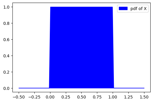
To reiterate the example given by Eric Jang, lets say you have a
continuous uniform random variable
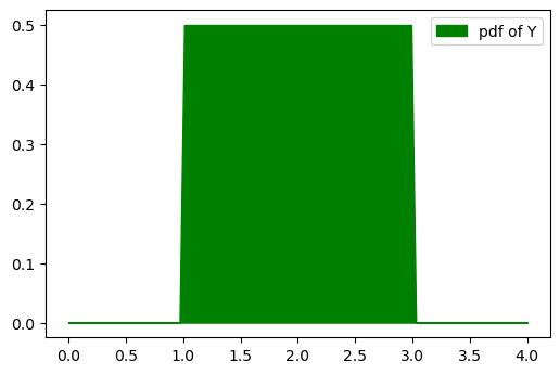
Let's say we give 
What would this distribution look like for

But can we prove this mathematically? Yes!
This is an example in 1D, but using change of variables theorem to
determine changes in probability distributions is the basis for
normalizing flows. The term
Code for 1D Example:
Defining the problem setting and solution in code might seem trivial if we know the answers already. But I found it a helpful exercise before expanding this idea to a 2 or more dimensional setting.
1 | # let's say we have a valid probability distribution where x is between [0,1] and p(x) = 1 |
1 | # now we know that if x is being projected by f(x), then px will be projected by 1/2 |
Normalizing Flows in 2D with Jax
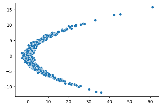
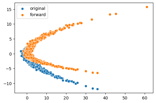
Let's define the same 2D dataset as Eric Jang's problem. We generate
1024 samples, and each sample has 2 points. There is a relationship
between the two points; to create a generative model, we want to find a
series of invertible functions which can untangle the "complicated"
relationships, and project each point to a unimodal normal distribution.
If successful, generating new samples is trivial: we take 2 samples from
a gaussian distribution and stack them as
1 | # define a target distribution |
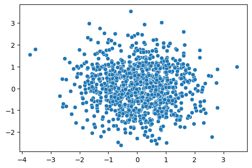
Regardless of your target distribution, after going through the flow, you want to final distribution to be a multi-variable normal distribution with no covariance/correlation. We assume the marginal distribution of each point after the transformations to be normal, and calculate the loss based on this assumption. This means that during training, the parameters of the functions are adjusted such that the points are projected into a multi-variate normal distribution, so something like this:
But how do we calculate this loss value? This is a critical step that
did not click with me right away. If my explanation isn't clear makes
sure to read one of the recommended posts mentioned early on. Let's
assume the flow only has 1 function,
We know that
In the next section, we'll write the code for this process :)
Defining Functions
We implement leakyRelu and realNVP, two common functions/layers used in normalizing flows. When defining layers, we have to define how it transforms an input, and also how to calculate the log determinant of the jacobian (LDJ). LDJs are passed through and added up in every layer, and are needed to calculated the projected probabilities. The probabilities are then used to calculate the loss of the network.
Relu
In a LeaklyRelu layer, if an input
Here,
1 | # using Flax's nn module |
You can visualize the effect of the layer.
1 | # initialize an lru layer |
 Inspecting the the
 params and LDJ values
should look something like this: 1
2
3
4
5
6
7FrozenDict({
params: {
alpha: DeviceArray([0.73105997], dtype=float32),
},
})
ldj list: [-0.31325978 -0.31325978 0. ... -0.31325978 -0.31325978
0. ]
where the outputs can take 3 values: 0,
Coupling Layers
A coupling layer is a layer where a subset of points in a sample (so
either
This setup allows for coupling, or transformation of some points
according to the value of other points. But we actually do not need to
know the inverse of the neural network, or whatever method we use to
calculate
I've modified an example provided by University of Amsterdam deep
learning course for the 2D example. A simple neural network (also called
a hyper-network) generates the scale and transform parameters for one of
the two points based on the value of the other. The coupling layer then
transforms the sample and calculates the LDJ. 1
2
3
4
5
6
7
8
9
10
11
12
13
14
15
16
17
18
19
20
21
22
23
24
25
26
27
28
29
30
31
32
33
34
35
36
37
38
39
40
41
42
43
44
45
46
47
48# modified from https://uvadlc-notebooks.readthedocs.io/en/latest/tutorial_notebooks/JAX/tutorial2/Introduction_to_JAX.html
# and https://uvadlc-notebooks.readthedocs.io/en/latest/tutorial_notebooks/JAX/tutorial11/NF_image_modeling.html
class SimpleNet(nn.Module):
num_hidden : int # Number of hidden neurons
num_outputs : int # Number of output neurons
def setup(self):
self.linear1 = nn.Dense(features=self.num_hidden)
self.linear2 = nn.Dense(features=self.num_outputs)
def __call__(self, x):
# Perform the calculation of the model to determine the prediction
x = self.linear1(x)
x = nn.tanh(x)
x = self.linear2(x)
return x
class CouplingLayer(nn.Module):
network : nn.Module # NN to use in the flow for predicting mu and sigma
mask : np.ndarray # Binary mask where 0 denotes that the element should be transformed, and 1 not.
c_in : int # Number of input channels
layer_type = "Scale and Shift"
def setup(self):
self.scaling_factor = self.param('scaling_factor',
nn.initializers.zeros,
(self.c_in,))
def __call__(self, z, ldj, rng, reverse=False):
# Apply network to masked input
z_in = z * self.mask
nn_out = self.network(z_in)
s, t = nn_out.split(2, axis=-1)
# Stabilize scaling output
s_fac = jnp.exp(self.scaling_factor).reshape(1, -1)
s = nn.tanh(s / s_fac) * s_fac
# Mask outputs (only transform the second part)
s = s * (1 - self.mask)
t = t * (1 - self.mask)
# Affine transformation
if not reverse:
# Whether we first shift and then scale, or the other way round,
# is a design choice, and usually does not have a big impact
z = (z + t) * jnp.exp(s)
ldj += s.sum(axis=[1])
else:
z = (z * jnp.exp(-s)) - t
ldj -= s.sum(axis=[1])
return z, ldj, rng
MultiLayer Network
We want to create a model with multiple layers, train it, and sample from it when we are done training. This is very simple to do with the networks we defined in flax, and the optimizers provided by optax . The sampling function could be even simpler if we didn't want to see the intermediate transformations. Notice that during sampling, we simply generate two points from a normal distribution and pass it back through the flows.
Architecture
1 | # multi layer network |
The PointsFlow model just needs a list of flow layers,
we've already defined Relu and Coupling layers. Notice that the mask
variable takes on the values of [1,0] or [0,1] every other layer.
1 | flow_layers = [] |
Training and Sampling
Now we need to define the loss calculation and optimizer. I found that adamw worked much better than SGD and adam. The loss function is where we calculate the negative log loss, which requires an understanding of the change of variable rules which was briefly discussed earlier. Try to derive it yourself on paper to make sure you understand how it works (Lilian Wang's blog was very helpful for me in this regard)
1 | optimizer = optax.adamw(learning_rate=0.0001) |
Finally, we define a train_step function. If you have a GPU, the
jitted function runs incredibly fast. 1
2
3
4
5
6
7
8
9
10
11
12
13
def train_step(state,rng,batch):
rng, init_rng = jax.random.split(rng,2)
grad_fn = jax.value_and_grad(loss_calc, # Function to calculate the loss
argnums=1, # Parameters are second argument of the function
has_aux=True # Function has additional outputs, here rng. Which you don't even need now that I think about it.
)
# Determine gradients for current model, parameters and batch
(loss,rng), grads = grad_fn(state, state.params, rng, batch)
# Perform parameter update with gradients and optimizer
state = state.apply_gradients(grads=grads)
# Return state and any other value we might want
return state, rng, loss
Training is simple and very fast if you have a GPU.
1
2
3
4
state = model_state
for i in range(50000):
state,rng,loss = train_step(state,rng,X)
print("iter %d patience %d loss %f"%(i,patience, loss) , end="\r")
And so is sampling: 1
2
3
4
5layers = ["random sample"] + [model.flows[i].layer_type for i in range(len(model.flows))][::-1] # names of generation layers (backward order of training layers)
for i,out in enumerate(mid_layers):
sns.scatterplot(x= out[:,0], y = out[:,1],label = "out of" + layers[i])
plt.show()